Features
Distributed Tracing
Monitor request flows with OpenTelemetry
Acontext traces requests through API, Core, database, cache, storage, and LLM calls using OpenTelemetry and Jaeger.
What's Traced
- HTTP requests
- Database queries
- Redis cache operations
- S3 storage operations
- RabbitMQ messages
- LLM embedding/completion calls
View Traces
Access traces from the dashboard:
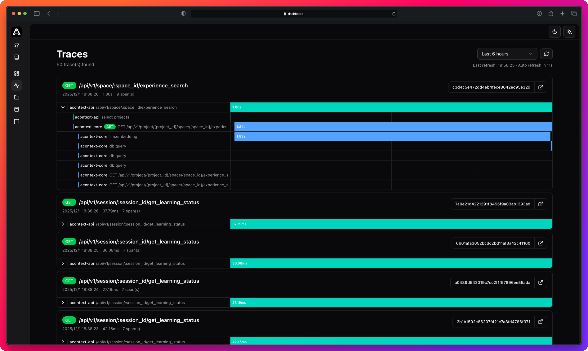
- Time filtering: 15min, 1h, 6h, 24h, 7d
- Auto-refresh: Every 30 seconds
- Service colors: Teal (api), Blue (core)
- Jaeger link: Click trace ID for detailed view
Configuration
Core (Python):
TELEMETRY_ENABLED=true
TELEMETRY_OTLP_ENDPOINT=http://localhost:4317
TELEMETRY_SAMPLE_RATIO=1.0
API (Go):
telemetry:
  enabled: true
  otlp_endpoint: "localhost:4317"
  sample_ratio: 1.0
Use sampling ratio < 1.0 in production (e.g., 0.1 for 10%) to reduce storage costs.
Next Steps
Last updated on